凡例を枠外に配置する方法 [matplotlib]

Matplotlib の凡例はデフォルトではプロット領域内に配置されますが、場合によっては枠外に配置することで、グラフの可読性を向上させることができます。本記事では、Matplotlib で凡例を枠外に配置する方法について詳しく解説します。

bbox_to_anchor を使って凡例を枠外に配置する

Matplotlib では、bbox_to_anchor 引数を使用することで、凡例をプロットの枠外に配置することができます。

基本的な使い方 (枠外右上に表示)

import matplotlib.pyplot as plt
import numpy as np

# データの作成
x = np.linspace(0, 10, 100)
y1 = np.sin(x)
y2 = np.cos(x)

# グラフの描画
fig, ax = plt.subplots()
ax.plot(x, y1, label='sin(x)')
ax.plot(x, y2, label='cos(x)')

# 凡例を枠外に配置
ax.legend(loc='upper left', bbox_to_anchor=(1, 1))

# レイアウト調整
plt.tight_layout()
plt.show()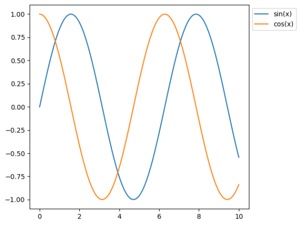

bbox_to_anchor の詳細

• loc='upper left' は凡例の基準点を指定します。
• bbox_to_anchor=(1,1) により、凡例をプロットの右上の外側に配置します。
• 第一引数（1）は x 座標（右端）
• 第二引数（1）は y 座標（上端）

枠外下中央

凡例をプロットの下部に配置する場合は、以下のように bbox_to_anchor を調整します。

# 凡例上部中央(upper center)をプロット下中央(0.5, -0.1)に配置
ax.legend(loc='upper center', bbox_to_anchor=(0.5, -0.1), ncol=2)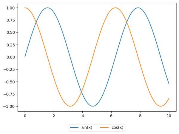

ncol=2として、凡例を横に並べています。

枠外右下

枠外右下にしたいときは、凡例の左下(lower left)を、プロットの右下(1,0)に指定します。

# プロット枠外右下
ax.legend(loc='lower left', bbox_to_anchor=(1, 0))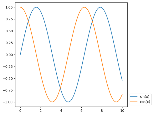

枠外上中央

凡例を枠外上中央に置くには、凡例中央下を、プロット中央上に配置します。

ax.legend(loc='lower center', bbox_to_anchor=(0.5, 1.05), ncol=2)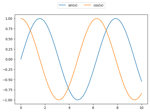

このように bbox_to_anchor を適切に設定することで、凡例の位置を自由にカスタマイズできます。

複数のサブプロットがあるとき

複数のサブプロットがある場合、ax.legend()やplot.legend()ではなくfig.legend() を使うことで図全体の枠外に凡例を配置できます。

fig, axs = plt.subplots(2, 1, figsize=(6, 6))

for ax in axs:
    ax.plot(x, y1, label='sin(x)')
    ax.plot(x, y2, label='cos(x)')

# 全体の凡例を枠外に配置
fig.legend(loc='upper center', bbox_to_anchor=(0.5, 1.1), ncol=2)

plt.tight_layout()
plt.show()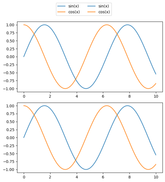

[補足] 余白を調整する

凡例を枠外に配置するとき、余白が不十分でレイアウトが崩れることがあります。そのときは、tight_layout() や constrained_layout=True 、subplots_adjust() を使用するとレイアウトの調整が可能です。

tight_layout()

tight_layout() は、プロット内の要素間の間隔を自動的に調整して、適切なレイアウトを作成する機能です。簡単な調整に適しています。

fig, ax = plt.subplots()
ax.plot(x, y1, label='sin(x)')
ax.plot(x, y2, label='cos(x)')
ax.legend(loc='upper left', bbox_to_anchor=(1, 1))

# 自動レイアウト調整
plt.tight_layout()
plt.show()

constrained_layout=True

constrained_layout=True を指定すると、プロット内の要素（軸、タイトル、凡例など）が自動で適切に配置され、重ならないように調整されます。サブプロットが多い場合に有効です。

fig, ax = plt.subplots(constrained_layout=True)
ax.plot(x, y1, label='sin(x)')
ax.plot(x, y2, label='cos(x)')
ax.legend(loc='upper left', bbox_to_anchor=(1, 1))
plt.show()

• 凡例を枠外に配置した場合でも、プロットのサイズが自動的に調整され、全体が見やすくなります。
• tight_layout() よりも高度なレイアウト調整が可能です。

subplots_adjust()

subplots_adjust() を使うと、プロットのマージンを手動で調整できます。上の２つの方法でうまくいかず、手動で指定したいときに使用します。

fig, ax = plt.subplots()
ax.plot(x, y1, label='sin(x)')
ax.plot(x, y2, label='cos(x)')
ax.legend(loc='upper left', bbox_to_anchor=(1, 1))

# 手動でマージンを調整
plt.subplots_adjust(right=0.75)
plt.show()

tight_layout() vs subplots_adjust() vs constrained_layout

まとめ

Matplotlib で凡例を枠外に配置するには、

• bbox_to_anchor を使ってカスタム位置を指定
• fig.legend() を利用してサブプロット全体の凡例を作成
• レイアウト調整は、constrained_layout=True 、tight_layout() で自動調整、または subplots_adjust() で手動調整

これらの方法を組み合わせることで、見やすいグラフを作成できます。